AdaBoost vs Gradient Boosting: How Combining Weak Learners Beats Any Single Tree

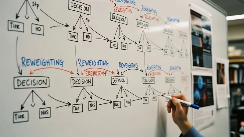
A single decision tree is a weak learner. Given a classification problem with any real complexity — like separating rare signal from overwhelming background at the LHC — one tree will underperform. It is too simple to capture the full structure of the separation boundary.

The insight behind boosting is that you do not need a single powerful model. You need many weak ones, combined. This idea traces back to a question posed by Kearns and Valiant in the late 1980s: can a collection of classifiers, each only slightly better than random guessing, be combined into one that is arbitrarily accurate? Schapire proved in 1990 that the answer is yes. Freund and Schapire then turned that proof into a practical algorithm: AdaBoost (Freund and Schapire, 1997, JCSS 55(1), 119--139), which won the Godel Prize.

AdaBoost: reweight the mistakes

AdaBoost works by training a sequence of weak classifiers — typically shallow decision trees with just a few leaves (often called "stumps" when limited to depth 1). After each tree is trained:

1. Events that the tree misclassified get higher weights.
2. Events that the tree classified correctly get lower weights.
3. The next tree is trained on the reweighted sample, so it focuses on the events the previous trees got wrong.

The final prediction is a weighted vote of all trees, where each tree's vote is weighted by how accurate it was overall.

from sklearn.ensemble import AdaBoostClassifier
from sklearn.tree import DecisionTreeClassifier

# Each weak learner is a shallow tree (depth 1 = stump).
ada = AdaBoostClassifier(
    estimator=DecisionTreeClassifier(max_depth=1),
    n_estimators=200,
    learning_rate=0.5,
    random_state=42,
)
ada.fit(X_train, y_train)
scores = ada.predict_proba(X_test)[:, 1]

The key mechanism is adaptive reweighting. Early trees handle the easy events; later trees concentrate on the hard cases near the decision boundary.

Gradient boosting: fit the residuals

Gradient boosting generalises the same idea but replaces the explicit reweighting with a more flexible framework. Instead of reweighting events, each new tree fits the residual errors (technically, the negative gradient of a loss function) of the ensemble built so far.

For classification with log-loss:

1. Start with a constant prediction (the log-odds of the class prior).
2. Compute the residual: the difference between the true label and the current predicted probability for each event.
3. Fit a shallow tree to those residuals.
4. Add that tree to the ensemble (scaled by the learning rate).
5. Repeat.

from sklearn.ensemble import GradientBoostingClassifier

gbc = GradientBoostingClassifier(
    n_estimators=300,
    max_depth=3,
    learning_rate=0.1,
    subsample=0.8,       # stochastic gradient boosting
    random_state=42,
)
gbc.fit(X_train, y_train)
scores = gbc.predict_proba(X_test)[:, 1]

The advantage is generality: any differentiable loss function works. XGBoost (Chen and Guestrin, 2016, KDD) extended this with second-order gradient information and built-in regularisation, becoming the default boosted decision tree implementation across HEP and industry.

Why the ensemble beats a single deep tree

A single deep tree can, in principle, model any decision boundary. Why not just grow one large tree?

Because a deep tree overfits. It partitions the training data into tiny leaves that capture statistical noise. This is the bias-variance tradeoff: a deep tree has low bias but high variance.

Boosting takes the opposite approach. Each tree is shallow — high bias, low variance. The ensemble reduces bias by combining many trees additively. The learning rate controls how aggressively each tree contributes; smaller values require more trees but regularise the ensemble more strongly.

AdaBoost vs gradient boosting in practice

For most HEP classification tasks, the two algorithms produce comparable results. Gradient boosting is more commonly used today because:

• It supports arbitrary loss functions (AdaBoost is tied to exponential loss).
• Stochastic gradient boosting (subsample < 1) adds a regularisation mechanism that AdaBoost lacks.
• XGBoost's implementation is fast, memory-efficient, and supports built-in handling of missing values.

Both algorithms share the core principle: an ensemble of weak learners, trained sequentially, each correcting the errors of its predecessors.

The bottom line

You do not need every mathematical detail to use these algorithms effectively. But understanding the mechanism — sequential correction, shallow trees, additive combination — tells you why tree depth, learning rate, and number of estimators are the knobs that control your classifier's bias-variance balance.

For the full progression from single trees through boosting to a validated, production-ready classifier, start with the free Module 1 and the Classifier Roadmap.

Educational material. It does not replace the internal review and approval procedures of your experiment's collaboration.