Watch a Boosted Decision Tree Beat Rectangular Cuts in One Plot
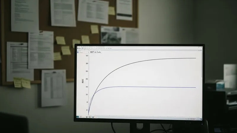
You've probably been told that boosted decision trees beat rectangular cuts. It's easier to believe when you watch it happen on a plot you generated yourself. This post is a single, runnable example — about 30 lines — that you can paste into a notebook right now.
The setup: two correlated observables
Imagine two discriminating variables where signal and background overlap, and — crucially — the separation runs along a diagonal, not along either axis. This is the situation rectangular cuts handle badly: a box in variable space can't follow a diagonal boundary without throwing away good signal or letting in background.
import numpy as np
from sklearn.ensemble import GradientBoostingClassifier
from sklearn.model_selection import train_test_split
from sklearn.metrics import roc_curve, auc
import matplotlib.pyplot as plt

rng = np.random.default_rng(42)
n = 20000

# Background: broad blob centred low. Signal: shifted along a diagonal.
bkg = rng.multivariate_normal([0.0, 0.0], [[1.0, 0.6], [0.6, 1.0]], n)
sig = rng.multivariate_normal([1.4, 1.4], [[1.0, 0.6], [0.6, 1.0]], n)

X = np.vstack([bkg, sig])
y = np.concatenate([np.zeros(n), np.ones(n)])
Xtr, Xte, ytr, yte = train_test_split(X, y, test_size=0.5, random_state=0)
The rectangular-cut baseline
A rectangular cut keeps events above a threshold in both variables. We sweep the threshold and trace out the efficiency–rejection trade-off — the cut-based ROC.
# Sweep a common threshold on both variables (the classic rectangular cut).
thresholds = np.linspace(-3, 4, 200)
cut_tpr, cut_fpr = [], []
for t in thresholds:
    passed = (Xte[:, 0] > t) & (Xte[:, 1] > t)
    cut_tpr.append(np.mean(passed[yte == 1]))   # signal efficiency
    cut_fpr.append(np.mean(passed[yte == 0]))   # background acceptance
cut_auc = auc(cut_fpr, cut_tpr)
The BDT
Now train a gradient-boosted decision tree on the same two variables and score the held-out sample. Note we evaluate on Xte — events the model never trained on.
bdt = GradientBoostingClassifier(n_estimators=200, max_depth=3, learning_rate=0.1)
bdt.fit(Xtr, ytr)
scores = bdt.predict_proba(Xte)[:, 1]
fpr, tpr, _ = roc_curve(yte, scores)
bdt_auc = auc(fpr, tpr)
The one plot
plt.figure(figsize=(5, 5))
plt.plot(cut_fpr, cut_tpr, label=f"Rectangular cuts (AUC={cut_auc:.3f})", lw=2)
plt.plot(fpr, tpr, label=f"Boosted decision tree (AUC={bdt_auc:.3f})", lw=2)
plt.plot([0, 1], [0, 1], "k--", alpha=0.3)
plt.xlabel("Background acceptance")
plt.ylabel("Signal efficiency")
plt.legend(loc="lower right")
plt.title("BDT vs rectangular cuts")
plt.tight_layout()
plt.savefig("bdt_vs_cuts.png", dpi=120)
Run it and you will see two curves. The boosted decision tree curve sits above and to the left of the rectangular-cut curve across the whole range — the same signal efficiency at lower background acceptance, or more signal at the same background. The area under the curve is visibly larger.
That gap is not a trick of this toy. It's the same effect Roe et al. measured on real particle identification: boosted decision trees improved signal efficiency by roughly 30–50% at equal background rejection compared with cuts (NIM A 543 (2005) 577–584). Rectangular cuts carve axis-aligned boxes; real signal and background separate along curved, correlated boundaries. The tree ensemble follows that boundary; the box cannot.
What this toy leaves out
This example is deliberately minimal, and everything it skips is exactly what turns a toy into a physics-grade analysis:
- Overtraining checks — here we evaluated on a held-out half, but you'd want the train/test overlay and a compatibility test.
- Data/MC agreement — a real boosted decision tree is only as trustworthy as its input modelling.
- Systematic uncertainties — the classifier is part of your measurement chain.
Those are the difference between "the classifier wins on a plot" and "the analysis survives review." If you want the full route — the six stages from this toy to a result you can defend in review, and the five mistakes reviewers check for — grab the free Module 1 and the Roadmap.
Educational material. It does not replace the internal review and approval procedures of your experiment's collaboration.
Want to go deeper?
Machine Learning for High Energy Physics: The Complete Course takes you from first principles to a defensible result in 6 structured modules. $97, 30-day guarantee.
See the course →Not ready yet? Grab Module 1 free →