Feature Engineering With Physics Observables

July 26, 2026 · 5 min read

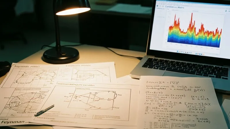
If you have spent years building analysis pipelines, you already have something most ML practitioners lack: deep physical intuition about which quantities are meaningful. Feature engineering in particle physics is not about inventing new variables from scratch — it is about systematically translating what you already trust into a form a classifier can use efficiently.

Why Feature Choice Matters More Than Model Choice

A gradient-boosted tree or neural network can, in principle, learn any decision boundary given enough data. In practice, feeding it raw detector outputs — track momenta components, calorimeter cell energies — makes that job much harder than necessary. The model must rediscover conserved quantities, Lorentz invariance, and detector geometry from scratch. Giving it physics observables ML features instead hands it the compressed, meaningful representation your field has refined over decades.

Poorly chosen inputs also hurt in subtler ways: they increase training time, demand more data to converge, and make it harder to diagnose what the classifier is actually doing. Investing time in feature engineering particle physics style pays dividends across all three.

Start With What You Already Plot

The first rule is conservative: begin with the variables you would put on a plot in a paper.

• Invariant masses — The invariant mass feature machine learning benefits are hard to overstate. A reconstructed mass like $m_{\ell\ell}$ or $m_{jj}$ compresses four four-vectors into one number that carries the dominant discriminating power for most resonance searches. Start here.
• Angular variables — $\Delta R$, $\Delta\phi$, $\cos\theta^*$, helicity angles. These encode the spin and decay topology of your signal and are often largely uncorrelated with pileup.
• Isolation and activity variables — $E_T^{\text{iso}}$, track multiplicity in a cone, lepton isolation. These separate prompt objects from fakes in ways that are physically motivated and detector-stable.
• Transverse momentum ratios — $p_T$ balance, $p_T$ fraction, thrust. Ratios are naturally dimensionless and often less sensitive to overall energy scale uncertainties.

These are your safest, most interpretable starting features. A classifier built on them is one you can explain to a referee.

Build Derived Features With Purpose

Once the obvious observables are in, think about what additional structure the classifier cannot easily construct itself.

Combine objects explicitly

If your signal involves a specific decay chain, reconstruct intermediate objects and compute their properties. For a $H \to WW^* \to \ell\nu\ell\nu$ analysis, the dilepton invariant mass and the angle between the leptons are far more useful to the model than the six individual lepton four-momentum components separately.

Encode asymmetries and orderings

Quantities like the signed $\eta$ difference between two jets, or the ratio of leading to subleading $p_T$, capture asymmetry information that symmetric inputs lose. If the physics is not symmetric under a swap, the features should not be either.

Use event-level summaries

Scalar sums ($H_T$, $S_T$), missing transverse energy significance, and sphericity encode global event shape. These matter especially when the signal populates a distinct region of phase space that is not captured by any single object.

Be cautious with high-level combinations

The more complex a derived variable, the more assumptions you bake in. Prefer variables with a clear physical meaning over ones that look empirically discriminating on a training sample — the latter are the route to overtraining, the ML equivalent of overfitting a chi-square to statistical fluctuations.

Practical Steps Before Training

1. Visualise each feature's signal-to-background shape. A quick stack plot tells you whether a variable has any discriminating power at all. If signal and background overlap almost perfectly, the feature may not be worth including.

2. Check for correlations. Including five highly correlated versions of the same variable (e.g., multiple mass windows derived from the same four-vectors) does not add information but does add noise. Use a simple correlation matrix to prune redundancy.

3. Assess systematic sensitivity. Prefer features whose shapes are stable under your dominant systematic variations. A variable that shifts dramatically with jet energy scale uncertainty will force your model to learn a feature it cannot reliably extrapolate to data.

4. Normalise consistently. Tree-based models are scale-invariant, but neural networks are not. Apply the same normalisation derived from your training set to all subsequent sets — validation, test, and data.

5. Document everything. Feature engineering decisions are physics decisions. Note why each variable was included so the next person on the analysis (or you, six months later) can understand and reproduce your choices.

When to Let the Model Help

There is a complementary approach — letting a network learn directly from lower-level inputs like particle flow candidates — which is worth exploring once your physics-feature baseline is solid. Understanding where your high-level features succeed and fail tells you exactly what you might gain from going lower-level. The complete course covers both strategies in sequence, including hands-on exercises that walk through feature selection decisions on realistic HEP datasets. You can also preview the approach in the free Module 1 before committing.

For a deeper look at how these features feed into classifier training and evaluation, the full course curriculum covers ROC curves, working point selection, and systematic-aware training in the same physics-first language.

The features you trust in a paper are the features your classifier should trust first — build from there.