Getting Started With Machine Learning for LHC Analysis

July 26, 2026 · 5 min read

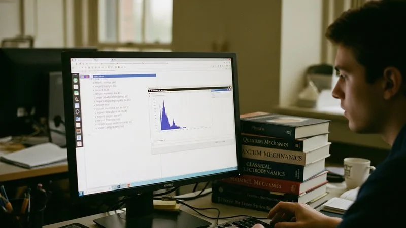
If you have spent years building a particle physics analysis and someone just told you to "add some ML to it," the advice probably landed with a thud. Machine learning for LHC analysis is genuinely powerful, but the path from that suggestion to a working classifier in your ntuple pipeline is not obvious. This guide lays out a practical, ordered roadmap so you can move from curious to capable without detours.

Understand What ML Actually Replaces

Before touching a single line of code, get clear on the conceptual trade. Classical LHC analysis builds cuts and discriminants from physics intuition — you choose observables, define selection windows, and tune them by hand. Machine learning replaces or augments that step by learning a discriminant directly from labelled examples. A boosted decision tree or a neural network is, at its core, a flexible function that maps a set of input observables (features) to a score. That score is optimised to separate signal from background.

If you already understand likelihood ratios and the Neyman–Pearson lemma, you understand what a well-trained classifier is approximating. That is your anchor. Everything else is engineering.

Step 1 — Get Comfortable With the Python Stack

Most practical machine learning particle physics tutorial material assumes Python, and the ecosystem is worth the investment. You need four libraries at minimum:

• NumPy and Pandas for array manipulation and tabular data
• Matplotlib for visualisation
• scikit-learn for classical ML models and evaluation utilities
• PyTorch or TensorFlow/Keras for neural networks

Start with scikit-learn. Its interface is consistent and its documentation is excellent. You can train a gradient-boosted tree on your ROOT ntuples (exported via uproot) in an afternoon. Get that working before worrying about deep learning.

Sub-step: bridge ROOT to Python

Use uproot to read .root files directly into NumPy arrays or Pandas DataFrames. No compiled C++ required. This single step removes most of the friction between your existing analysis infrastructure and the ML ecosystem.

Step 2 — Start With a Classifier You Can Explain

Resist the pull of large neural networks at the outset. A gradient-boosted decision tree — XGBoost or scikit-learn's GradientBoostingClassifier — trains quickly, is interpretable, and performs well on tabular physics data. It also fails loudly when something is wrong, which matters enormously when you are learning.

Train on Monte Carlo signal and background. Use a clean, well-understood signal region. Your goal at this stage is not to beat the state of the art; it is to build one full cycle: prepare data, train a model, evaluate it, and understand what it learned.

Step 3 — Learn to Evaluate Correctly

ROC curves are your primary evaluation tool. In physics language, the ROC curve is simply efficiency versus background rejection plotted as a function of threshold — something you already know how to read. The area under the ROC curve gives an aggregate summary of performance, but always look at the curve itself. A classifier that is excellent at high signal efficiency may be poor at the high-purity end you actually care about.

The early trap to avoid: evaluating on the training sample. This is the ML version of fitting a chi-square with too many free parameters and reporting the minimum as a result. Split your data into training, validation, and test sets before touching the model. Keep the test set locked until you have finalised all choices.

Overtraining — the ML term for what you would call overfitting — is detectable: the ROC on the training sample looks better than on the validation sample. Monitor this gap throughout training.

Step 4 — Connect ML Outputs to Physics

A classifier score is not a physical observable until you understand its systematic behaviour. Before using any ML discriminant in a fit, ask:

• Does the score distribution agree between data and MC in a control region?
• How does the score respond to variations of the dominant systematic uncertainties?
• Does the model learn features that are well-modelled, or does it exploit poorly-modelled tails?

Feature importance tools (SHAP values are particularly useful here) help you see which observables the model leans on. If it is leaning heavily on a variable you know is poorly modelled, that is a physics problem, not an ML problem.

Where to Go Deeper

The steps above will carry you through a first working analysis. When you are ready to move into graph neural networks, anomaly detection, or fast inference for triggers, the learning curve steepens — but the foundations you have built transfer directly.

For a structured path through all of this, the full HEP ML course covers the complete journey from tabular classifiers to modern deep learning architectures, with examples drawn from collider physics throughout. If you want to sample it first, Module 1 is available free and gets you through the Python stack and your first classifier. For more on specific techniques relevant to LHC searches, the HEP ML blog has focused articles on topics like jet tagging, anomaly detection, and uncertainty-aware training.

Takeaway: the fastest way into machine learning for LHC analysis is one complete, honest training cycle — real data, honest evaluation, and a model you can explain to a collaborator.

References

Radovic, A., Williams, M., Rousseau, D., Kagan, M., Bonacorsi, D., Himmel, A., Aurisano, A., Terao, K., & Wongjirad, T. (2018). Machine learning at the energy and intensity frontiers of particle physics. Nature, 560, 41-48.

Albertsson, K., et al. (2018). Machine Learning in High Energy Physics Community White Paper. Journal of Physics: Conference Series, 1085, 022008. arXiv:1807.02876.