Signal vs Background: Machine-Learning Classification in HEP

July 26, 2026 · 5 min read

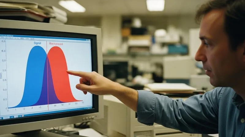
If you have spent any time staring at a signal region in a particle physics analysis, you already know the frustration: your signal looks like a needle, your background looks like a haystack, and rectangular cuts on a handful of variables never seem to carve away enough background without also throwing away most of your signal. Machine learning reframes this problem in a way that is both natural and powerful — and it is worth understanding exactly how before you start training anything.

The Classification Framing

Signal background classification is, at its core, a binary decision: for each event, does it look more like signal or more like background? That is exactly the task that supervised classification algorithms are designed to solve.

In ML language, each event is a data point described by a vector of features — what physicists call observables. Transverse momenta, invariant masses, angular separations, b-tagging scores: all of these become input features. The classifier's job is to learn a function that maps an event's feature vector to a single number, typically a score between 0 and 1, representing how signal-like the event is. You then cut on that score rather than on individual variables.

The key insight is that a well-trained classifier effectively combines all of your input variables into a single discriminant, exploiting correlations among them that a sequence of rectangular cuts would miss entirely.

Why ML Often Outperforms Rectangular Cuts

Rectangular cuts live in axis-aligned boxes. If your signal occupies a diagonal band in the plane of two correlated variables, a box will either include too much background or exclude too much signal — there is no way around it. A classifier is not constrained to axis-aligned boundaries. It can learn curved, high-dimensional decision surfaces that hug the actual signal topology.

The deeper reason is dimensionality. As you add more discriminating observables, the volume of possible phase space grows exponentially. Optimizing cuts by hand in five or ten dimensions is practically impossible. A neural network, boosted decision tree, or gradient-boosted classifier explores that full space during training.

This is also why signal background separation machine learning methods have become standard across collider experiments. For analyses searching for rare decays, exotic signatures, or new resonances with small cross-sections, recovering even a modest improvement in signal efficiency at fixed background rejection can translate directly into improved discovery sensitivity.

How to Set It Up

Step 1 — Assemble your training samples

You need labelled examples: simulated signal events (label = 1) and simulated background events (label = 0). Use the same generator and reconstruction pipeline you trust for your analysis. Make sure the kinematic distributions in your simulation are a reasonable match to data before you proceed — a classifier trained on a mismodelled simulation will learn the wrong boundaries.

Be deliberate about which phase-space region you train on. If you train inclusively but evaluate in a restricted signal region, performance can degrade. Some analysts train in a sideband-to-signal-region workflow, which also helps with decorrelation.

Step 2 — Choose your features carefully

Start with variables that have known physics motivation for discrimination: invariant masses, isolation quantities, angular variables, jet substructure observables. Avoid variables that are poorly modelled in simulation — the classifier will try to use them, and you will have a hard time validating performance in data.

For a primer on thinking through feature selection in an HEP context, the full course at HEP ML walks through this systematically, including worked examples with realistic datasets.

Step 3 — Train, validate, and watch for overtraining

Split your simulated sample into training, validation, and test sets before you touch anything. Overtraining in ML is exactly what it sounds like in statistics: the model fits the noise in the training sample and generalises poorly. Monitor your loss curve on the validation set alongside the training set. If they diverge, you are overtraining — reduce model capacity, add regularisation, or get more data.

Step 4 — Evaluate with physics metrics

After training, the standard ML metric is the ROC curve — which is, in physics language, the signal efficiency versus background rejection curve. A point on the ROC curve answers the question: "If I accept this fraction of signal events, what fraction of background events do I also accept?" That is exactly efficiency versus purity, a language every physicist already speaks.

Integrate the ROC curve to get the AUC (area under the curve) as a summary statistic, but always look at the full curve: your analysis may care specifically about operating at very high background rejection, and the AUC averages over regions you do not care about.

For event classification in particle physics, the final output score is not automatically your cut variable. Consider whether you need to decorrelate the score from the invariant mass you are fitting — a topic covered in detail in the course modules.

A Note on Validation in Data

Training on simulation and deploying on data requires care. Validate your classifier output distribution in a control region where you know the composition. Check that signal and background sculpting in the discriminant distribution match your expectation before unblinding.

Signal background separation with machine learning is not magic — it is a principled way to exploit the full information content of your events rather than projecting it down to a handful of one-dimensional cuts. Start with a simple baseline, validate rigorously, and build from there.

References

Baldi, P., Sadowski, P., & Whiteson, D. (2014). Searching for exotic particles in high-energy physics with deep learning. Nature Communications, 5, 4308. arXiv:1402.4735.