Why Rectangular Cuts Fail When Your Variables Are Correlated

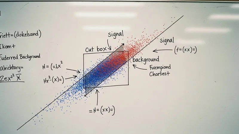
Rectangular cuts are the oldest selection tool in particle physics. You require variable_1 > threshold_1 AND variable_2 > threshold_2, and whatever survives is your candidate sample. For decades, this worked well enough.

It stops working when your variables are correlated — and in a real analysis, they almost always are.

The geometry of the problem

A rectangular cut defines an axis-aligned box in variable space. If signal and background separate cleanly along each axis independently, the box captures the signal region efficiently.

But suppose your best separation runs along a diagonal — for example, the difference x1 - x2 separates signal from background, but neither x1 nor x2 alone does. A rectangular cut in (x1, x2) space cannot follow that diagonal boundary. It must choose: keep the box tight and lose signal, or open the box wide and accept background.

This is not a hypothetical. In HEP, discriminating variables are routinely correlated. Kinematic variables share the same underlying four-momenta. PID likelihoods depend on overlapping detector subsystems. Isolation and impact parameter both respond to the same displaced topology.

A concrete example

import numpy as np

rng = np.random.default_rng(42)
n = 50000

# Signal: offset along a diagonal. Background: centred at origin.
# Strong correlation (rho = 0.7) in both populations.
cov = [[1.0, 0.7], [0.7, 1.0]]
bkg = rng.multivariate_normal([0.0, 0.0], cov, n)
sig = rng.multivariate_normal([1.2, 1.2], cov, n)

# Rectangular cut: keep events with x1 > 0.6 AND x2 > 0.6
cut_mask_sig = (sig[:, 0] > 0.6) & (sig[:, 1] > 0.6)
cut_mask_bkg = (bkg[:, 0] > 0.6) & (bkg[:, 1] > 0.6)

print(f"Rectangular cut — signal eff: {cut_mask_sig.mean():.3f}, "
      f"bkg eff: {cut_mask_bkg.mean():.3f}")

# Diagonal cut: keep events with (x1 + x2) / sqrt(2) > 0.85
diag_sig = (sig[:, 0] + sig[:, 1]) / np.sqrt(2)
diag_bkg = (bkg[:, 0] + bkg[:, 1]) / np.sqrt(2)
diag_mask_sig = diag_sig > 0.85
diag_mask_bkg = diag_bkg > 0.85

print(f"Diagonal cut    — signal eff: {diag_mask_sig.mean():.3f}, "
      f"bkg eff: {diag_mask_bkg.mean():.3f}")

Run this and you will find the diagonal cut achieves comparable signal efficiency at substantially lower background acceptance. The rectangular cut wastes statistical power because it is fighting the geometry of the correlation.

The curse of dimensionality makes it worse

In two dimensions, the rectangular cut is merely inefficient. In ten or twenty dimensions — common in a modern analysis — the problem compounds. The volume of an axis-aligned box in d dimensions scales as the product of the side lengths. As you add variables, the fraction of the hypervolume that actually contains signal shrinks exponentially relative to the box that encloses it.

Roe et al. (2005) measured this directly on MiniBooNE particle identification data: a boosted decision tree improved signal efficiency by roughly 30--50% at the same background rejection compared with optimised rectangular cuts (NIM A 543(2--3), 577--584). The gain came precisely from the tree ensemble's ability to partition the space along non-axis-aligned, nonlinear boundaries.

What a multivariate method does differently

A boosted decision tree does not choose one global boundary. It builds hundreds of small, axis-aligned splits — individually weak — and combines them. The ensemble boundary can follow curves, diagonals, and islands in variable space. It adapts to correlations automatically because each successive tree focuses on the events the previous trees got wrong.

This is why "adding more variables" helps a boosted decision tree but often hurts rectangular cuts. Each new variable gives the tree more directions to split; each new variable gives the rectangular cut another axis-aligned wall that may not align with the true separation surface.

When rectangular cuts are still fine

Rectangular cuts remain appropriate for pre-selection — loose requirements that reduce combinatorics or enforce trigger acceptance, where optimal efficiency is not the goal. They are also easier to validate systematically, since each cut maps to a single variable.

The point is not that cuts are wrong. It is that, for the final signal selection in a competitive analysis, they leave signal on the table that a multivariate classifier recovers.

If you want to see this progression from cuts to a validated boosted decision tree classifier — including the overtraining checks and systematic uncertainty propagation that make it survive review — grab the free Module 1 and the Classifier Roadmap.

Educational material. It does not replace the internal review and approval procedures of your experiment's collaboration.